Linear Regression
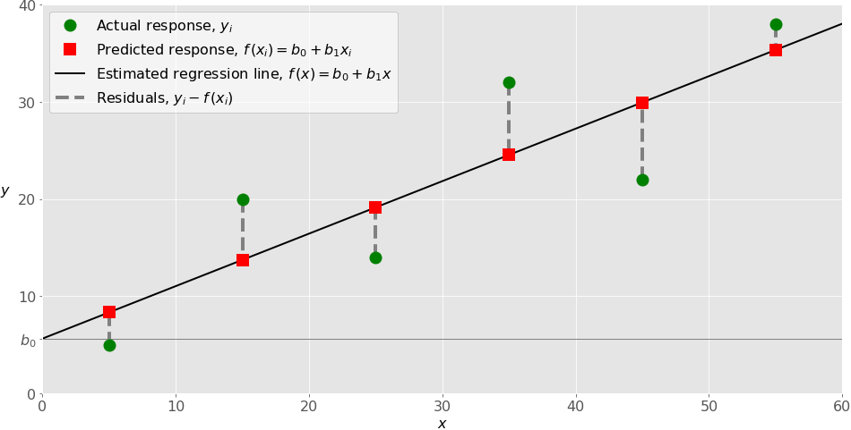
Simple model with "x" is the predictor value (input variable, independent variable), and y is the output (predicted variable, also the dependent variable)
Computes the input in the equation y = mx + b, and gives an output
Simple model with "x" is the predictor value (input variable, independent variable), and y is the output (predicted variable, also the dependent variable)
Computes the input in the equation y = mx + b, and gives an output
Linear Regression
Prediction Equation: y^ = θ0 + θ1x1 + θ2x2 + ..... θnxn
Use case for linear regression
It is a simple model, use the equation for input and you will get the expected output.
Polynomial regression
Polynomial regression is capable of finding relationships between features when we have to use multiple features for a prediction. A simple linear regression model can not do that, so when dealing with multiple features polynomial regression is better.
The degree of the polynomial PolynomialFeatures(degree=d), the array containing the features is transformed from an array containing n features to (n+d)!/d!n! features.
Polynomial should be used when a straight line can't be drawn through your data. Polynomial regression helps to transform that data to a more of a linear regression model.
Gradient descent is an algorithm commonly used to find the minimum of a function. It is a first-order iterative optimization algorithm, which means it uses the gradient of the function to update its position in search space. The process is repeated until the minimum is reached or a stopping criterion is met.
To minimize the cost function
Gradient descent is a widely used algorithm in various machine learning applications, including linear regression, logistic regression, neural networks, and deep learning. It is a versatile algorithm that can be applied to a broad range of optimization problems.
There are several reasons why gradient descent is a popular choice for optimization problems:
Random initialization is a common practice in gradient descent. It involves picking an arbitrary set of starting values for the parameters of the model being optimized. This is done because if the starting point is always the same, the algorithm may converge to a local minimum instead of the global minimum of the cost function.
Batch gradient descent is a type of gradient descent that uses the entire training dataset to calculate the gradient of the cost function in each iteration. This can be computationally expensive for large datasets.
Stochastic gradient descent is a type of gradient descent that uses a single training example to calculate the gradient of the cost function in each iteration. This can be more efficient than batch gradient descent for large datasets, but it can also lead to more fluctuations in the learning process.
Mini-batch gradient descent is a type of gradient descent that uses a small subset of the training dataset (mini-batch) to calculate the gradient of the cost function in each iteration. This is a compromise between batch gradient descent and stochastic gradient descent, offering a balance between computational efficiency and smoothness of the learning process.
| Overfitting: Variance | Underfitting: Bias |
|---|---|
| Performs well during training, but NOT on testing data | Does NOT perform well during training and testing |
| Does NOT generalize well in the real world | High bias, fails to capture complexity on the data |
| Performs well during training, BUT bad Cross validation | Too simple, model not trained long enough |
| Occurs when: model is Too complex | How to address:
|
| Need to regularize (L1 and L2, Elastic NET) | Too simple of a model |
For both Linear and Logistic Regression:
Metrics For Logistic Regression and Classification:
Why regularization: When a model is performing well on the training set, but performs poorly on the testing data, that is that the model is overfitting. When a model is overfitting that is when regularization is needed. Remember, overfitting is that the model has high variance on the testing set.
Say for example we have very little training data, and the model learns the training instances well, but for the testing set the predictions are off and the graph of the predicted outcomes looks a little bit scattered. The testing set has some degree of variance. To address this we need to introduce some bias, and that is where regularization comes in.
By introducing some bias, the model that is overfitting can now generalize the test dataset better. This is done in different ways based on each cost function from which regularization method you choose.
The hyperparameter lambda is needed to control the learning rate, the higher the lambda value, the less sensitive the model becomes to the training data. Eventually as lambda goes higher, the slope of the regression line just goes down to 0. What you will end up with is a straight horizontal line that goes through the mean of the data.
Lasso Regression:
L1 will shrink less important features down to 0, thus doing feature selection. If you have a lot of features and aren’t sure which to select, L1 regularization will shrink the less important features down to 0, thus performing feature selection.
Cost Function: \( J(\mathbf{w}) = \frac{1}{2m} \sum_{i=1}^{m} (h_{\mathbf{w}}(\mathbf{x}^{(i)}) - y^{(i)})^2 + \lambda \sum_{j=1}^{n} |w_j| \)
L1 will shrink less important features down to 0, thus doing feature selection. If you have a lot of features and aren’t sure which to select, L1 regularization will shrink the less important features down to 0, thus performing feature selection.
Cost Function: \( J_{\text{L2}}(\mathbf{w}) = \frac{1}{2m} \sum_{i=1}^{m} (h_{\mathbf{w}}(\mathbf{x}^{(i)}) - y^{(i)})^2 + \frac{\lambda}{2} \sum_{j=1}^{n} w_j^2 \)
What L2 does is it shrinks coefficients for the features that are playing less of a role to to predict y asymptotically close to 0. This helps deal with multicollinearity, thus effectively reducing the weight of non-important features. L2 does not shrink coefficients down to 0, but get them asymptotically close to 0, L2 therefore won’t remove any features.
Regularization term is added to the MSE. This should only be added to the cost function during training. Lambda will control the regularization, lambda represents the learning rate. Ridge is sensitive to the scale of the model, so be sure to scale your data (i.e. standard scaler).
Early stopping
Used in softmax to prevent overfitting
When validation error reaches a minimum: